이미지 핸들링 수업 1~3주차

대학원 수업/이미지 핸들링

이미지 핸들링 수업 1~3주차

Tech코알라 2025. 10. 22. 23:33

# matplotlib로 이미지 표시 (BGR→RGB 변환 필수)
plt.imshow(cv2.cvtColor(img, cv2.COLOR_BGR2RGB))
plt.axis('off')
plt.show()

* 해당 내용은 서울시립대학교 도시빅데이터융합학과 이미지 핸들링 수업을 재구성한 내용입니다.

2025학년도 2학기 이미지 핸들링 수업은 말 그대로 이미지를 다루는 수업입니다. 특히 openCV, CLIP, YOLO 등을 다루게 되는데 해당 내용을 강사님의 경험에 맞춰서 번호판 인식에 맞춰서 수업을 진행하실 예정이라고 하십니다.

1주차 : opencv 사용법

OpenCV(Open Source Computer Vision Library)는 컴퓨터 비전과 머신러닝을 위한 오픈소스 라이브러리입니다.

주요 특징

실시간 이미지 처리: 빠른 속도로 이미지/영상 처리 가능
다양한 기능: 이미지 읽기/쓰기, 색상 변환, 필터링, 객체 감지 등
크로스 플랫폼: Windows, Linux, macOS, Android, iOS 지원
다중 언어 지원: Python, C++, Java 등

BGR 색상 순서

OpenCV는 BGR(Blue-Green-Red) 순서를 사용 (일반적인 RGB와 반대)
이는 역사적인 이유로 채택된 규칙

python에서 opencv를 설치하는 방법은 아래와 같다.

pip3 install opencv-python # python에서 opencv 설치

# 라이브러리 임포트
import cv2
import numpy as np
from matplotlib import pyplot as plt

# 이미지 읽기
img = cv2.imread('test.bmp')

# 이미지는 numpy 배열 (3차원: 높이, 너비, 채널)
print(type(img))  # <class 'numpy.ndarray'>

# 이미지 저장
cv2.imwrite('test.jpg', img)  # 손실 압축
cv2.imwrite('test2.bmp', img)  # 무손실
cv2.imwrite('test2.png', img)  # 무손실

# BGR 채널 확인
blue_img = cv2.imread('blue_grid.bmp')   # [255, 0, 0]
green_img = cv2.imread('green_grid.bmp') # [0, 255, 0]
red_img = cv2.imread('red_grid.bmp')     # [0, 0, 255]

# BGR → RGB 변환
img_rgb = cv2.cvtColor(img_color, cv2.COLOR_BGR2RGB)

# RGB → BGR 변환 (BGR2RGB와 동일한 동작)
img_bgr = cv2.cvtColor(img_color, cv2.COLOR_RGB2BGR)

# BGR → Grayscale
img_gray = cv2.cvtColor(img_color, cv2.COLOR_BGR2GRAY)

# Grayscale → BGR (3채널로 변환하되 색상 정보 없음)
img_gray_to_color = cv2.cvtColor(img_gray, cv2.COLOR_GRAY2BGR)

# matplotlib로 이미지 표시 (BGR→RGB 변환 필수)
plt.imshow(cv2.cvtColor(img, cv2.COLOR_BGR2RGB))
plt.axis('off')
plt.show()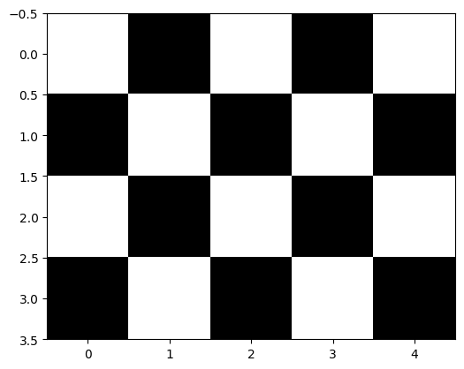

#flip
aeroplane_flip = cv2.flip(myimage, 0)   # 상하 반전
aeroplane_flip = cv2.flip(myimage, 1)   # 좌우 반전
aeroplane_flip = cv2.flip(myimage, -1)  # 상하좌우 반전

#rotate 
aeroplane_rotate = cv2.rotate(myimage, cv2.ROTATE_90_CLOCKWISE)        # 시계방향 90도
aeroplane_rotate = cv2.rotate(myimage, cv2.ROTATE_180)                 # 180도
aeroplane_rotate = cv2.rotate(myimage, cv2.ROTATE_90_COUNTERCLOCKWISE) # 반시계방향 90도

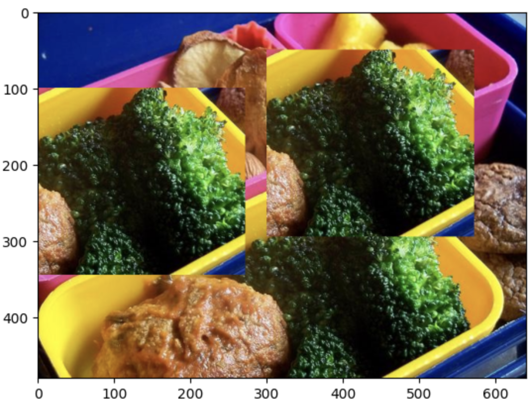
#crop
# 배열 슬라이싱으로 이미지 일부 추출
broccoli = img[235:480, 278:550]  # [높이_시작:끝, 너비_시작:끝]

# 다른 위치에 붙여넣기
img[100:345, 0:272] = broccoli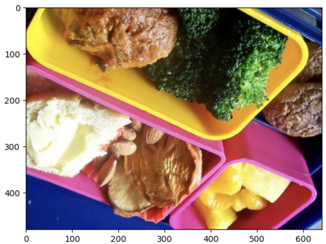

#커스텀 이미지 만들기 
height, width, channel = myimage.shape

with open('myimage.txt', 'w') as f:
    f.write(f"{height}\n{width}\n{channel}\n")
    
    for h in range(height):
        for w in range(width):
            for c in range(channel):
                f.write(f"{myimage[h][w][c]}\n")
                
#텍스트 파일에서 이미지 복원
with open('myimage.txt', 'r') as f:
    height = int(f.readline().strip())
    width = int(f.readline().strip())
    channel = int(f.readline().strip())
    
    myimg = np.zeros((height, width, channel))
    
    for h in range(height):
        for w in range(width):
            for c in range(channel):
                myimg[h][w][c] = int(f.readline().strip())
    
    # uint8 타입 변환 필수 (0-255 범위)
    myimg = myimg.astype(np.uint8)

핵심 개념 정리

이미지 = 숫자 배열: 이미지는 단순히 숫자들이 담긴 NumPy 배열
3차원 구조: (높이, 너비, 채널) 형태
BGR 순서: OpenCV는 BGR 채널 순서 사용
픽셀 값 범위: 0~255 (uint8 타입)
손실/무손실 압축: JPG(손실) vs BMP/PNG(무손실)
배열 조작 = 이미지 조작: 슬라이싱, 인덱싱으로 이미지 편집 가능

2주차 : Annotation, 이미지 라벨링

딥러닝 모델은 함수와 같습니다. 입력(이미지)을 받아서 출력(인식 결과)을 내놓습니다. 1주차에서 이미지가 숫자라는 것을 배웠다면, 2주차에서는 출력(라벨)도 숫자라는 점을 이해할 수 있습니다.

MNIST 데이터셋

손글씨 숫자를 인식하는 가장 기본적인 데이터셋입니다.

28x28 크기의 흑백 이미지 70,000장
학습용: 60,000장
테스트용: 10,000장

from tensorflow.keras.datasets import mnist

(x_train, y_train), (x_test, y_test) = mnist.load_data()

print(f'학습용 입력이미지: {len(x_train)}장')
print(f'테스트용 입력이미지: {len(x_test)}장')

# 샘플 시각화
plt.figure(figsize=(8, 8))
for i in range(16):
    plt.subplot(4, 4, i+1)
    plt.imshow(x_train[i], cmap='gray')
    plt.title(f"Label: {y_train[i]}")
    plt.axis('off')
plt.show()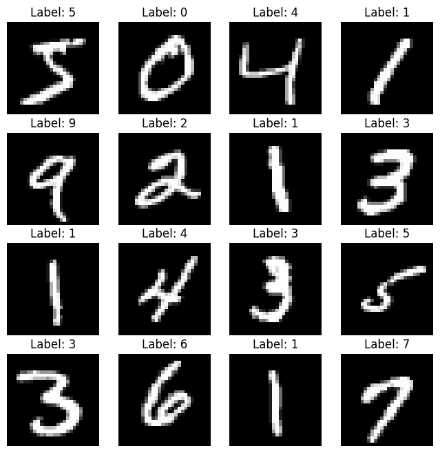

모델의 입력과 출력

입력 데이터 전처리:

28x28 흑백 이미지 → 28x28x1 (채널 추가)
정규화: 픽셀 값 0과 1 사이의 소수점 값

x_train = x_train.reshape(-1, 28, 28, 1).astype('float32') / 255.0
x_test = x_test.reshape(-1, 28, 28, 1).astype('float32') / 255.0

출력 데이터 변환:

단순히 "7"이라는 숫자가 아닌 * 10개의 확률 값으로 변환 (One-hot encoding 개념) 예시:

손글씨가 7일 경우 : [0.0001, 0.0002, 0.0001, 0.0001, 0.0002, 0.0001, 0.0001, 0.9989, 0.0001, 0.0001] 와 같이

→ 7번 인덱스가 가장 높은 확률(0.9989)을 가짐

왜 100%가 아닌가?

AI 모델은 오차가 완전히 0이 될 수 없음
오차를 0에 가깝게 만드는 방향으로 학습
실용적으로는 99.89%면 충분히 정확한 예측

모델 학습 및 예측

import tensorflow as tf
from tensorflow.keras import layers, models

# CNN 모델 정의
model = models.Sequential([
    layers.Conv2D(16, (3,3), activation='relu', input_shape=(28,28,1)),
    layers.MaxPooling2D((2,2)),
    layers.Conv2D(32, (3,3), activation='relu'),
    layers.MaxPooling2D((2,2)),
    layers.Flatten(),
    layers.Dense(128, activation='relu'),
    layers.Dense(10, activation='softmax')  # 10개 클래스 출력
])

model.compile(optimizer='adam',
              loss='sparse_categorical_crossentropy',
              metrics=['accuracy'])

# 학습
model.fit(x_train, y_train, epochs=5, validation_split=0.2)

실전: 내가 그린 손글씨 인식시키기

import cv2
import numpy as np

# 1. 이미지 읽기 (흑백)
img = cv2.imread("my_handwriting_3.png", cv2.IMREAD_GRAYSCALE)

# 2. 전처리
img = cv2.resize(img, (28, 28))           # 크기 맞추기
img = img.astype("float32") / 255.0       # 정규화
img = img.reshape(1, 28, 28, 1)           # 배치 차원 추가

# 3. 예측
pred = model.predict(img)

# 4. 결과 확인
print("각 숫자별 확률:")
for i, p in enumerate(pred[0]):
    print(f"  숫자 {i}일 확률: {p:.6f}")

predicted_digit = np.argmax(pred[0])
print(f"\n예측 결과: {predicted_digit}")

주의사항: 배경색 문제

문제 상황:

MNIST는 검은 배경에 흰 글씨
우리가 그린 이미지는 보통 흰 배경에 검은 글씨
이 차이로 인해 인식률이 급격히 떨어짐

해결 방법 1: 이미지 반전

# 이미지 읽기 후 반전
img = cv2.imread("3.png", cv2.IMREAD_GRAYSCALE)
img = 255 - img  # 반전

# 시각화
plt.imshow(img, cmap='gray')
plt.show()

# 이후 동일한 전처리 과정
img = cv2.resize(img, (28, 28))
img = img.astype("float32") / 255.0
img = img.reshape(1, 28, 28, 1)

pred = model.predict(img)

해결 방법 2: 반전 데이터로 재학습

from tensorflow.keras.datasets import mnist
import numpy as np

# 1. 원본 데이터 로드
(x_train, y_train), (x_test, y_test) = mnist.load_data()

# 2. 반전 데이터 생성
x_train_inverted = 255 - x_train
x_test_inverted = 255 - x_test

# 3. 원본 + 반전 데이터 합치기
x_train = np.concatenate([x_train, x_train_inverted], axis=0)
y_train = np.concatenate([y_train, y_train], axis=0)  # 라벨은 동일

x_test = np.concatenate([x_test, x_test_inverted], axis=0)
y_test = np.concatenate([y_test, y_test], axis=0)

# 4. 정규화 및 학습
x_train = x_train.reshape(-1, 28, 28, 1).astype('float32') / 255.0
x_test = x_test.reshape(-1, 28, 28, 1).astype('float32') / 255.0

new_model = models.Sequential([...])  # 동일한 구조
new_model.compile(optimizer='adam',
                  loss='sparse_categorical_crossentropy',
                  metrics=['accuracy'])

new_model.fit(x_train, y_train, epochs=5, validation_split=0.2)

이제 흰 배경/검은 배경 모두에서 잘 작동하는 모델이 완성됩니다!

다른 객체 인식으로 확장

알파벳 인식 모델을 만든다면?

A → 0
B → 1
C → 2
...
Z → 25

→ 26개의 출력을 가진 모델 정의 → 가장 높은 확률을 가진 인덱스가 예측된 알파벳

동물 분류 모델을 만든다면?

고양이 → 0
개 → 1
새 → 2

→ 3개의 출력을 가진 모델

핵심 개념: 어떤 객체든 숫자로 매핑하면 분류 문제로 해결 가능!

객체 탐지(Object Detection)

분류(Classification)와 달리, 객체의 위치까지 찾아야 합니다.

COCO128 데이터셋 다운로드

import urllib.request
import zipfile

url = "https://ultralytics.com/assets/coco128.zip"
save_path = "coco128.zip"

# 다운로드
urllib.request.urlretrieve(url, save_path)

# 압축 해제
with zipfile.ZipFile(save_path, 'r') as zip_ref:
    zip_ref.extractall()

객체 라벨링: 위치도 숫자다!

객체의 위치를 표현하는 방법은 여러 가지가 있습니다.

YOLO 형식 (정규화된 좌표):

<class_index> <x_center> <y_center> <width> <height>

각 값의 의미:

class_index: 객체 클래스 번호 (0=사람, 1=자전거, 2=자동차 등)
x_center: 박스 중심의 x 좌표 / 이미지 너비
y_center: 박스 중심의 y 좌표 / 이미지 높이
width: 박스 너비 / 이미지 너비
height: 박스 높이 / 이미지 높이

왜 정규화를 할까?

이미지 크기와 무관하게 0~1 사이의 값으로 표현
색상 정보를 255로 나눈 것과 같은 원리
다양한 해상도의 이미지에 대응 가능

라벨 파일 시각화

import os
import cv2
import matplotlib.pyplot as plt

# 경로 설정
img_dir = "coco128/images/train2017"
label_dir = "coco128/labels/train2017"

img_name = "000000000009.jpg"
img_path = os.path.join(img_dir, img_name)
label_path = os.path.join(label_dir, img_name.replace(".jpg", ".txt"))

# 이미지 로드
img = cv2.imread(img_path)
img_h, img_w, _ = img.shape

# 라벨 파일 읽기
with open(label_path, 'r') as f:
    for line in f:
        class_id, x_center, y_center, width, height = map(float, line.strip().split())
        
        # 정규화된 좌표를 픽셀 좌표로 변환
        x_center *= img_w
        y_center *= img_h
        width *= img_w
        height *= img_h
        
        # 좌상단, 우하단 좌표 계산
        xmin = int(x_center - width / 2)
        ymin = int(y_center - height / 2)
        xmax = int(x_center + width / 2)
        ymax = int(y_center + height / 2)
        
        # 바운딩 박스 그리기
        cv2.rectangle(img, (xmin, ymin), (xmax, ymax), (0, 255, 0), 2)
        cv2.putText(img, str(int(class_id)), (xmin, ymin-10),
                    cv2.FONT_HERSHEY_SIMPLEX, 0.9, (0, 255, 0), 2)

plt.figure(figsize=(12, 8))
plt.imshow(cv2.cvtColor(img, cv2.COLOR_BGR2RGB))
plt.axis('off')
plt.show()

COCO 클래스 정의

# COCO 80개 클래스
names = {
    0: "person", 1: "bicycle", 2: "car", 3: "motorcycle", 4: "airplane",
    5: "bus", 6: "train", 7: "truck", 8: "boat", 9: "traffic light",
    # ... (총 80개)
}

라벨링 형식 비교

Pascal VOC 형식:

<xmin>100</xmin>  <!-- 픽셀 좌표 -->
<ymin>150</ymin>
<xmax>250</xmax>
<ymax>300</ymax>
<name>person</name>

YOLO 형식:

0 0.5 0.5 0.3 0.4  # class x_center y_center width height (정규화)

변환 공식:

# YOLO → Pascal VOC
xmin = (x_center - width/2) * image_width
ymin = (y_center - height/2) * image_height
xmax = (x_center + width/2) * image_width
ymax = (y_center + height/2) * image_height

# Pascal VOC → YOLO
x_center = (xmin + (xmax - xmin)/2) / image_width
y_center = (ymin + (ymax - ymin)/2) / image_height
width = (xmax - xmin) / image_width
height = (ymax - ymin) / image_height

실습: 라벨링 도구 사용하기

labelImg 설치 (Python 3.9 권장):

# Ubuntu 예시
git clone https://github.com/HumanSignal/labelImg.git
cd labelImg
conda create -y -n label python=3.9
conda activate label
sudo apt-get install pyqt5-dev-tools
pip install -r requirements/requirements-linux-python3.txt
make qt5py3

# 실행
python labelImg.py

labelImg 사용법:

Open Dir: 이미지 폴더 선택
Create RectBox: 바운딩 박스 그리기
클래스 이름 입력
Save: 자동으로 YOLO 형식 .txt 파일 생성

핵심 개념 정리

라벨링도 숫자: 클래스명 → 숫자 인덱스, 위치 → 정규화된 좌표
정규화의 중요성: 이미지 크기와 무관하게 0~1 범위로 통일
형식의 다양성: YOLO, Pascal VOC 등 다양한 형식 존재
수작업의 번거로움: labelImg 같은 도구로도 시간 소모가 큼
자동화의 필요성: 이미지 핸들링 기술로 라벨링 자동화 가능

3주차 : Perspective Transform (원근 변환)

번호판 인식 시스템의 핵심 기술인 원근 변환을 배웁니다. 기울어진 번호판을 정면으로 보이게 만들고, 다른 차량 이미지에 합성하는 과정을 실습합니다.

학습 목표

기울어진 번호판을 정면 뷰로 변환 (Deskew)
정면 번호판을 다른 차량에 합성
Annotation 좌표도 함께 변환

데이터 준비

# 차량 이미지 2장 다운로드
!wget -O license_plate1.jpg "https://storage.googleapis.com/kagglesdsdata/datasets/686454/1203932/images/Cars134.png?..."
!wget -O license_plate2.jpg "https://storage.googleapis.com/kagglesdsdata/datasets/686454/1203932/images/Cars120.png?..."

import cv2 as cv
import numpy as np
from matplotlib import pyplot as plt

# 이미지 로드 및 확인
license_plate1_image = cv.imread('license_plate1.jpg')
license_plate2_image = cv.imread('license_plate2.jpg')

plt.figure(figsize=(12, 6))
plt.subplot(1, 2, 1)
plt.imshow(cv.cvtColor(license_plate1_image, cv.COLOR_BGR2RGB))
plt.title('Car 1 (with plate)')

plt.subplot(1, 2, 2)
plt.imshow(cv.cvtColor(license_plate2_image, cv.COLOR_BGR2RGB))
plt.title('Car 2 (target)')
plt.show()

Perspective Transform의 원리

핵심 개념:

Source points (원본 4개 꼭짓점)

Destination points (목표 4개 꼭짓점)

변환 행렬(Transformation Matrix)

Source Points → [Transformation Matrix] → Destination Points

OpenCV는 4개의 점 대응 관계만 알면 자동으로 변환 행렬을 계산해줍니다!

# 1. 원본 번호판의 4개 꼭짓점 (수동으로 찾음)
source_pts = np.float32([
    [80, 151],   # 좌상단
    [131, 155],  # 우상단
    [131, 173],  # 우하단
    [80, 165]    # 좌하단
])

# 2. 목표 좌표 (정면으로 펼친 직사각형)
deskewed_pts = np.float32([
    [0, 0],       # 좌상단
    [520, 0],     # 우상단
    [520, 110],   # 우하단
    [0, 110]      # 좌하단
])

# 3. 변환 행렬 계산
deskew_matrix = cv.getPerspectiveTransform(source_pts, deskewed_pts)

# 4. 변환 적용
license_plate1_image = cv.imread('license_plate1.jpg')
deskewed_plate = cv.warpPerspective(
    license_plate1_image, 
    deskew_matrix, 
    (520, 110)  # 출력 이미지 크기
)

# 5. 결과 확인
plt.figure(figsize=(10, 4))
plt.subplot(1, 2, 1)
plt.imshow(cv.cvtColor(license_plate1_image[140:180, 70:140], cv.COLOR_BGR2RGB))
plt.title('Original (Skewed)')

plt.subplot(1, 2, 2)
plt.imshow(cv.cvtColor(deskewed_plate, cv.COLOR_BGR2RGB))
plt.title('Deskewed (Front View)')
plt.show()

결과: 기울어진 번호판이 깔끔한 정면 뷰로 변환됩니다!

Step 2: 정면 번호판 → 다른 차량에 합성

# 1. 목표 위치의 4개 꼭짓점 (차량2의 번호판 위치)
target_pts = np.float32([
    [159, 179],  # 좌상단
    [248, 180],  # 우상단
    [248, 198],  # 우하단
    [159, 198]   # 좌하단
])

# 2. 정면 뷰 → 목표 위치 변환 행렬
warp_matrix = cv.getPerspectiveTransform(deskewed_pts, target_pts)

# 3. 변환 적용
warped_plate = cv.warpPerspective(
    deskewed_plate, 
    warp_matrix, 
    (400, 265)  # 차량2 이미지 크기
)

plt.imshow(cv.cvtColor(warped_plate, cv.COLOR_BGR2RGB))
plt.title('Warped to Target Position')
plt.show()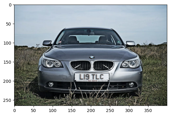

Step 3: 마스크를 이용한 자연스러운 합성

단순히 이미지를 덮어쓰면 네모난 경계가 보입니다. 마스크를 사용하여 번호판 영역만 정확히 합성합니다.

# 1. 정면 번호판과 같은 크기의 흰색 마스크 생성
deskewed_mask = np.zeros_like(deskewed_plate)
deskewed_mask.fill(255)  # 모든 픽셀을 흰색으로

plt.imshow(cv.cvtColor(deskewed_mask, cv.COLOR_BGR2RGB))
plt.title('Deskewed Mask')
plt.show()

# 2. 마스크에도 동일한 변환 적용
mask_image = cv.warpPerspective(
    deskewed_mask, 
    warp_matrix, 
    (400, 265)
)

plt.imshow(cv.cvtColor(mask_image, cv.COLOR_BGR2RGB))
plt.title('Warped Mask')
plt.show()

# 3. 마스크 영역만 합성
license_plate2_image = cv.imread('license_plate2.jpg')

# 마스크가 흰색(255)인 부분만 번호판 픽셀로 교체
license_plate2_image[mask_image == (255, 255, 255)] = \
    warped_plate[mask_image == (255, 255, 255)]

plt.figure(figsize=(12, 8))
plt.imshow(cv.cvtColor(license_plate2_image, cv.COLOR_BGR2RGB))
plt.title('Final Result')
plt.axis('off')
plt.show()

# 저장
cv.imwrite('result.jpg', license_plate2_image)

결과: 차량1의 번호판이 차량2에 자연스럽게 합성됩니다!

Annotation 좌표도 함께 변환하기

이미지만 변환하면 끝이 아닙니다. Annotation 좌표도 함께 변환해야 합니다!

원본 Annotation 읽기 (Pascal VOC 형식)

import xml.etree.ElementTree as ET

annotations = []

# XML 파일 파싱
tree = ET.parse('original.xml')
root = tree.getroot()

# 이미지 크기 정보
size = root.find('size')
image_width = int(size.find('width').text)
image_height = int(size.find('height').text)
depth = int(size.find('depth').text)

# 객체 정보 추출
objects = root.findall('object')
for obj in objects:
    name = obj.find('name').text
    bndbox = obj.find('bndbox')
    xmin = int(bndbox.find('xmin').text)
    ymin = int(bndbox.find('ymin').text)
    xmax = int(bndbox.find('xmax').text)
    ymax = int(bndbox.find('ymax').text)
    
    annotations.append({
        'name': name,
        'xmin': xmin,
        'ymin': ymin,
        'xmax': xmax,
        'ymax': ymax
    })

바운딩 박스 좌표 변환

import cv2 as cv
import numpy as np

# 이전에 사용한 변환 행렬
source_pts = np.float32([[80, 151], [131, 155], [131, 173], [80, 165]])
target_pts = np.float32([[159, 179], [248, 180], [248, 198], [159, 198]])
warp_matrix = cv.getPerspectiveTransform(source_pts, target_pts)

transformed_annotations = []

for ann in annotations:
    # 바운딩 박스의 4개 꼭짓점
    corners = np.float32([
        [ann['xmin'], ann['ymin']],  # 좌상단
        [ann['xmax'], ann['ymin']],  # 우상단
        [ann['xmax'], ann['ymax']],  # 우하단
        [ann['xmin'], ann['ymax']]   # 좌하단
    ]).reshape(-1, 1, 2)
    
    # 좌표 변환
    transformed_corners = cv.perspectiveTransform(corners, warp_matrix)
    
    # 변환된 좌표에서 최소/최대값 추출
    transformed_corners = transformed_corners.reshape(-1, 2)
    new_xmin = int(np.min(transformed_corners[:, 0]))
    new_ymin = int(np.min(transformed_corners[:, 1]))
    new_xmax = int(np.max(transformed_corners[:, 0]))
    new_ymax = int(np.max(transformed_corners[:, 1]))
    
    transformed_annotations.append({
        'name': ann['name'],
        'xmin': new_xmin,
        'ymin': new_ymin,
        'xmax': new_xmax,
        'ymax': new_ymax
    })

새로운 Annotation XML 파일 생성

import xml.etree.ElementTree as ET
from xml.dom import minidom

# XML 루트 생성
annotation = ET.Element('annotation')

# 파일명
filename = ET.SubElement(annotation, 'filename')
filename.text = 'result.jpg'

# 이미지 크기
size = ET.SubElement(annotation, 'size')
width = ET.SubElement(size, 'width')
height = ET.SubElement(size, 'height')
depth_elem = ET.SubElement(size, 'depth')
width.text = str(image_width)
height.text = str(image_height)
depth_elem.text = str(depth)

# 객체 정보 추가
for ann in transformed_annotations:
    obj = ET.SubElement(annotation, 'object')
    
    name = ET.SubElement(obj, 'name')
    name.text = ann['name']
    
    bndbox = ET.SubElement(obj, 'bndbox')
    xmin = ET.SubElement(bndbox, 'xmin')
    ymin = ET.SubElement(bndbox, 'ymin')
    xmax = ET.SubElement(bndbox, 'xmax')
    ymax = ET.SubElement(bndbox, 'ymax')
    
    xmin.text = str(ann['xmin'])
    ymin.text = str(ann['ymin'])
    xmax.text = str(ann['xmax'])
    ymax.text = str(ann['ymax'])

# Pretty print를 위한 포맷팅
xml_str = minidom.parseString(ET.tostring(annotation)).toprettyxml(indent="  ")

# 파일 저장
with open('result.xml', 'w') as f:
    f.write(xml_str)

print("새로운 annotation 파일 생성 완료: result.xml")

변환된 바운딩 박스 시각화

license_plate2_image = cv.imread('license_plate2.jpg')

for ann in transformed_annotations:
    cv.rectangle(
        license_plate2_image,
        (ann['xmin'], ann['ymin']),
        (ann['xmax'], ann['ymax']),
        (0, 0, 255),  # 빨간색
        2
    )
    cv.putText(
        license_plate2_image,
        ann['name'],
        (ann['xmin'], ann['ymin'] - 10),
        cv.FONT_HERSHEY_SIMPLEX,
        0.9,
        (0, 0, 255),
        2
    )

plt.figure(figsize=(12, 8))
plt.imshow(cv.cvtColor(license_plate2_image, cv.COLOR_BGR2RGB))
plt.title('Transformed Bounding Box')
plt.axis('off')
plt.show()
```

### 주의사항: 왜곡 문제

**발견된 문제:**
* 변환 후 바운딩 박스 주변에 의도하지 않은 공간 발생
* 번호판의 **실제 4개 꼭짓점**이 아닌 **사각형 바운딩 박스**를 변환했기 때문

**원인:**
```
원본 (기울어진 번호판):
  [xmin, ymin] -------- [xmax, ymin]
       |                    |
       |  실제 번호판 영역    |
       |                    |
  [xmin, ymax] -------- [xmax, ymax]

기울어진 번호판의 실제 영역은 평행사변형인데, 직사각형 바운딩 박스로 근사하면 불필요한 배경이 포함됩니다.

해결 방안:

실제 4개 꼭짓점을 직접 라벨링: 더 정확하지만 수작업 필요
Segmentation 기법 사용: 픽셀 단위로 정확한 영역 추출
기울기 보정: Skew가 큰 경우 변환 전에 회전 보정

핵심 개념 정리

Perspective Transform: 4개 점 대응으로 원근 변환 가능
마스크 활용: 자연스러운 이미지 합성의 핵심
Annotation 변환: 이미지뿐 아니라 좌표도 함께 변환 필수
왜곡 주의: 바운딩 박스 변환 시 Skew 정도에 따라 오차 발생
실용적 응용: 번호판 인식, 문서 스캔 앱 등에 활용

이렇게 1~3주차 내용을 정리했습니다!

1주차: 이미지는 숫자
2주차: 라벨도 숫자
3주차: 좌표 변환도 숫자 연산

'대학원 수업 > 이미지 핸들링' 카테고리의 다른 글

이미지 핸들링 : 번호판 이미지 생성 총정리 (1)	2025.11.25
[이미지 핸들링] 6,7 주차 수업 내용 정리 (0)	2025.10.23
[이미지 핸들링] 4,5 주차 수업 내용 정리 (0)	2025.10.23

현재글이미지 핸들링 수업 1~3주차

코알라 오딧세이

전문연구요원으로 AI를 연구하고 있습니다. AI, IT, 일상 등에 대해서 이야기합니다.

Svelte, intel #npu #gaudi #llm, ㅎ, PagedAttention, vllm, llm #exaone #exaone-deep #resoning, 관광 #RAG #우수상,

Today :
Yesterday :

코알라 오딧세이